
During the season 2014/2015, Real Madrid’s striker position was covered by the frenchman Karim Benzema. As opposed to Mourinho’s philosophy of rotating the striker almost on a game by game basis, Carlo Ancelotti had Benzema starting every game and left Javier “Chicharito” Hernandez in the bench for the majority of the season. Benzema played 2,312 La Liga minutes while Hernandez played 859 minutes. One could assume Chicharito was not world class quality, but every time he jumped on the pitch, he responded by scoring. How can we determine which player deserved to be in the initial lineup?
Determining who is the better player can become a never ending opinion battle, so I’m focusing this analysis on who is the most effective striker. Where I define “most effective striker” as the player who has the highest probability of scoring, given the fact that he is included in the starting squad. The data comes from Squwawka and the module I’m experimenting with is the PyMC Python module.
A little bit of data wrangling before we begin… I build two dataframes including the date of the match and the goals scored for Benzema and Hernandez. These dataframes exclude games where the player was active for less than 10 minutes. This is because it is may just not enough time for the striker to perform.
As mentioned before, we want to calculate the probability of scoring at least one goal given that the player was included in the starting squad. The probability can be solved by using Bayes’ Rule as shown bellow:
\( P( k > 0 | Y= 1) = \frac{P( Y = 1 | k >0 ) \times P( k > 0)}{P( Y = 1 | k >0) \times P(K > 0) + P( Y = 1 | K =0) \times P(K=0)} \)
Where:
K: Number of Goals scored in game
Y=1: Starting game
Y=1: Entering as a substitute
From the equation above, it is clear we need to find the probability of scoring \( P(K>0 \) for Hernandez and Benzema. To do this, we will use the PyMC module.
To begin with, I set up my Ipython environmanet to load all these modules.
%matplotlib inline
import matplotlib.pyplot as plt
import pandas as pd
import datetime
import numpy as np
import scipy.stats as stats
import pymc as pm  #This is the Bayesian Analysis module, it's great!
The first step in the analysis is to define the probabiliy distribution we want to base our model on. The Poisson distribution is the most appropriate because it is discrete and gives attributes a higher probability to lower values of K. Keep in mind we are talking about soccer and alghough possible, it is rare when we see a player scoring multiple goals in one match. The parameter that differenciates Hernandez Poisson distribution from Benzema’s Poisson distribution is the \( \lambda \) parameter, and we now need to define it.
The \( \lambda \) parameter is what determines the shape of the distribution. A larger \( \lambda \), gives a greater probability for larger values of K. In our case, a larger \( \lambda \) will indicate a higher chance of scoring larger number of goals. We initially don’t know \( \lambda \), but we can begin by estimating it. Heuristically, I determined that the best distribution was an Exponential distribution with an \( \alpha \) parameter of the inverse of the mean. This is going to be our prior distribution for \( \lambda \).
#Prior
alpha = 1.0 / df['Goals/Game*'][0].mean()
lambda_CH = pm.Exponential('lambda_CB', alpha)
alpha = 1.0 / df['Goals/Game*'][1].mean()
lambda_KB = pm.Exponential('lambda_KB', alpha)

@pm.deterministic
def observed_proportion_CH(lambda_CH=lambda_CH):
    out = lambda_CH
    return out

@pm.deterministic
def observed_proportion_KB(lambda_KB=lambda_KB):
    out = lambda_KB
    return out
In the code above, we set our prior distribution PyMC varialbes for \( \lambda _{CH} \) and \( \lambda _{KB} \). We then used the @pm.deterministic decorator to indicate ovserved_proportion_CH and observed_proportion_KB as a deterministic function. (This is required to work with PyMC models)
The next step is to devlop a model. In the code below, the variable obsCH use the value paremter to mold the striker’s goal scoring distribution. Note that we “educate” our distribution with our data using the “value” parameter in the function.
obsCH = pm.Poisson("obsCH", observed_proportion_CH, observed=True, value=CH_red_df['GoalinGame'])
obsKB = pm.Poisson("obsKB", observed_proportion_KB, observed=True, value=df_Benzema['GoalinGame'])

model_CH = pm.Model([obsCH, lambda_CH, observed_proportion_CH, obsCH])
mcmc_CH = pm.MCMC(model_CH)
mcmc_CH.sample(40000, 15000)

model_KB = pm.Model([obsKB, lambda_KB, observed_proportion_KB, obsKB])
mcmc_KB = pm.MCMC(model_KB)
mcmc_KB.sample(40000, 15000)
At this point, we have sucessfuly defined a posterior distribution for our parameters \( \lambda _{CH} \) and \( \lambda _{KB} \). To extract samples, we use the following code:
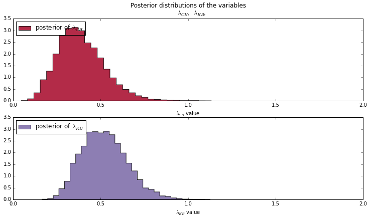
lambda_CH_samples = mcmc_CH.trace(lambda_CH)[:]
lambda_KB_samples = mcmc_KB.trace(lambda_KB)[:]
These parameters are shown in the graph below. \( \lambda _{KB} \) has a higher value than \( \lambda _{CH} \) on average. Using these parameters in a poisson distribution gives us the graph below.
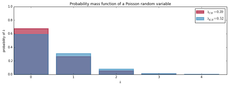
We could assume Benzema is more effective than Javier Hernandez, but we are missing one final step. We have ignored whether the player was a starter or a substitute. For the case of Benzema, no adjustment is necessary since he was never a substitute. For his case, the Bayesian equation is reduced to the tautology:
\( P( k > 0 ) = ( P( k > 0 ) \)
Where:
\( P( k > 0 ) = 43.46\% \)
This is not the case for Javier Hernandez. Hernandez played 19 games, 11 as a substitute player and 8 as a starter. He was a starter on 4 of the 5 times he scored and he was a starter on 4 of the 14 times he didn’t get his name on the scoreboard. Hence, Hernadez Probability Bayesian Equation:
\( P( k > 0 | Y= 1) = \frac{P( Y = 1 | k >0 ) \times P( k > 0)}{P( Y = 1 | k >0) \times P(K > 0) + P( Y = 1 | k =0) \times P(K=0)} \)
can be answered as:
\( P( k > 0 | Y= 1) = \frac{P( Y = 1 | k >0 ) \times P( k > 0)}{\frac{4}{5} \times P(K > 0) + \frac{4}{14} \times P(K=0)} \)
\( P( k > 0 | Y= 1) = 57.19\% \)
According to our anlysis, Hernandez is 13.73% more likely to score than the frenchman Karim Benzema when being in the starting eleven.
Upon showing this report to people, a common response was “Yes, Hernandez scores as a sub because the defense is tired”. So we’re now going to compare apples to apples and use only full game statistics.
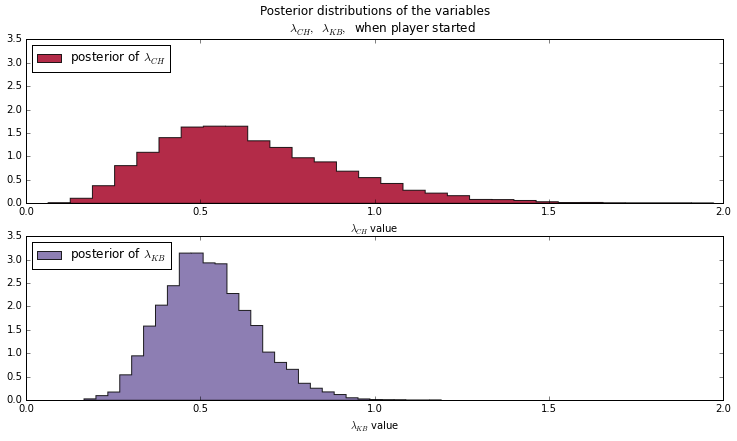
Notice, how Hernandez’ \( \lambda \) has wider tails than Benzema’s \( \lambda\). This is because we have less data for Hernandez (8 games vs Benzema’s 29 games) On the plot below, we appreciate the scoring probabilities of both. As we should expect from the \( \lambda \) parameters, Hernandez is more likely to score than Benzema.
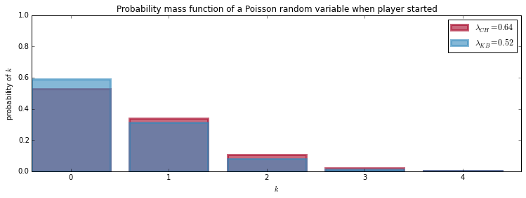
Hernadez has a 47.4% probability of scoring when starting a game and Benzema has a 40.8% probability of scoring.