I’m not trying to feed a fed horse (I had to) with this post, but there’s nothing more dangerous than drawing conclusions from a poorly excecuted AB test. This post is will detail the factors to consider when designing an AB Test and the reasoning behind each factor.

Null Hypothesis (\(H_{0})\)

Coming up with a hypothesis to test is the arguably the most important part of an experiment. There is nothing to test without a hypothesis. The Hypothesis we seek to reject is the Null Hypothesis. A common \(H_{0}\) for AB tests is \(\mu_{A}=\mu_{B}=\). Which states the mean of sample A is equal to the mean of sample B.

p-value

The p-value is a powerful statistic and typically if this value is lower than 0.05 we reject the Null Hypothesis. That is a very simplistic definition, as there is more to know about the p-value. Rathe than a magic number, we should think of the p-value as the probability of an event equal to or more extreme than the observed one occurring when the Null Hypothesis (\(H_{0})\) is TRUE. When the p-value is under 0.05, it means the event is unlikely to happen, thus we can reject the Null and accept an alternative hypothesis.

..but WAIT!!

Calculating the p-value is not enough. In fact, way before we calcualte the metric, we need to know how large our data sample should be and we should when running an experiment we need to complete the data acquisition stage before calculating p-values.

Consider the following example to

Toss Fair Coin Example

Imagine you want to test whether a coin is fair or not. You flip a coin 10000 times and after each toss count the cumulative number of times the coin landed on Head. Using the rbinom R function we simulate the tosses and we assign a probability of 50% for Heads. Now using the binom.test R function we check the p-value for when our (\(H_{0}) = 0.5 \). Since we assigned the probability of 50% we know the Null hypothesis is TRUE so we expect the p-value to be high.

set.seed(2)
n=10000
toss <- rbinom(n,1,prob=0.5)
p.values <- numeric(n)
erun<-numeric(n)
for (i in 5:n){
  p.values[i] <- binom.test(table(toss[1:i]),p=0.5)$p.value
  erun[i]<-i
}
df<-data.frame(erun,p.values)
df%>%ggplot(aes(x=erun,y=p.values))+geom_line()+
  geom_hline(yintercept=0.05,color='red',size=1,linetype='dashed',alpha=0.5)+
  labs(x = "Coin Flips", y = "p-value",
       title = "Change in p-value") +
  theme_bw() + theme(axis.text = element_text(size = 10), 
                     title = element_text(size = 10)) 

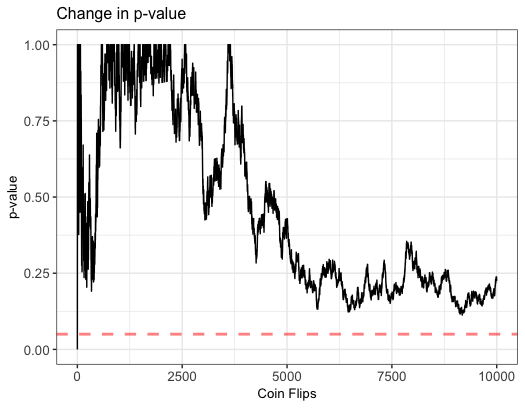
As we can see in the graph, the p-values are larger than the standard threshold of 0.05 throughout the duration of the experiment, but we can observe some large fluctuations. As we continue tossing more coins our p-value jumps all over. In this case, we accept the Null hypothesis at all time but it is possible to not be this lucky.

set.seed(22)
n=10000
toss <- rbinom(n,1,prob=0.5)
p.values <- numeric(n)
erun<-numeric(n)
for (i in 5:n){
  p.values[i] <- binom.test(table(toss[1:i]),p=0.5)$p.value
  erun[i]<-i
}

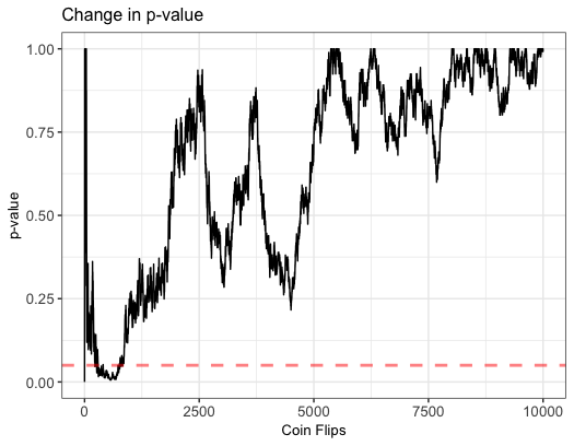
In this example, we repeated the experiment with the exact same parameters as the one above, but in this case, we do see our p-value fall under 0.05. As we continue to toss more coins, the p-value rises above the threshold. The lesson here is, the p-value is a strong metric but it’s only reliable whenever our sample size is large enough. If we peek early, we might draw erroneous conclusions.

Sample Size

We know we need a large enough sample size, but exactly how large? Well this depends on the effect we wish to detect, and the variance of our data. Detecting a small effect will increase our required sample size.

The following formula is commonly used to calculate a sample size

\(n = 16 \frac{\sigma^{2}}{\delta^2}\)

Where \( \delta\) is the minimum effect we wish to detect (Calculated as difference in sample means divided by pooled standard deviation). Also notice, having a large sample variance, will result in a large sample size needed.

If you’re an R user you can use the following to get a sample size:

library(pwr)
pwr.t.test(n=NULL,d=0.1, sig.level=0.05, power=0.8)

     Two-sample t test power calculation 

              n = 1570.733
              d = 0.1
      sig.level = 0.05
          power = 0.8
    alternative = two.sided

NOTE: n is number in *each* group

Power and sigificance level

Power is the probability of finding an effect when there is one. We can think of it as 1 - P(Type II error). It is standard to set this as 80% but this can change based on the nature of the experiment.

Significance level is the probability of finding an effect that is Not there. In other words, P(Type I error). The standard is to set this as 0.05.

Conclusion

So there you have it, AB testing is a very “simple” and powerful tecnnique, but we NEED to make sure we have enough data to draw conclusions. Immediately after writing our hypothesis, we need to calculate a minimum required sample size, and only if we know we can get the minimum sample size needed to detect an effect, we should proceed with the experiment.

Notes

• Type I error: occurs when we Reject a Null Hypothesis when it is True
• Type II error: occurs when we Fail to Reject the Null Hypothesis when it is False)