I compare the two wide receivers competing for the XWR starting position on the TEXAS Football 2017 season roaster. I use data from Dorian Leonard (Sr.) and Collin Johnson’s (So.) game day performances to see if there is a guy who is without a doubt ‘The Guy’. This study uses data up to the TCU game (11/04/2017).
Conversions in this study are defined by the following:
- If 1st or 2nd down: Receiver catches the ball and gains at least 3 yards (or Touchdown)
- If 3rd or 4th down: Receiver catches the ball gains the yards needed for the 1st down (or Touchdown)
Process
The technique used in the study is Bayesian Inference. I chose this, because of the difference in sample sizes between both players, and the fact that both sample sizes are rather small. I aim to find the ‘true’ conversion rate (cvr) for each receiver and then determine which receiver is better, based delta (\( cvr_A - cvr_B \)). To get satarted, I assignd a Uniform distribution as the prior , and then use observed data to model the posterior landscape. Posterior distribution plots are then produced via sampling (using NUTS) method.
XWR Receptions
| Player | Times Targeted | Conversions | Conversion Rate | Yrds Gained |
|---|---|---|---|---|
| Dorian Leonard | 25 | 13 | 52.0% | 126 |
| Collin Johnson | 66 | 34 | 51.5% | 575 |
To keep the plots kosher (and easy for me to recycle code) I’ll user the following nomenclature:
- A: Dorian Leonard (Sr.)
- B: Collin Johnson (So.)
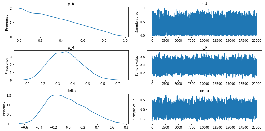
In the first two plots below, I show the probability distriution for the conversion rate of receiver A and B. The third plot, is the difference between A and B, in this case Dorian Leonard vs Collin Johnson.
The x-axis is the cvr which spans anywhere form 0 to 1, and the y-axis represents the times x occurred in the posterior sample. The peak in the plot, represents the ‘true’ conversion rate. This should read like any probability distribution graph; the highest point in the graph represents the most probable point.
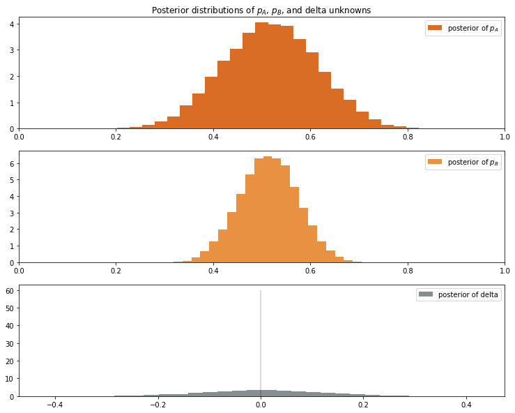
As we can see, both receivers’ conversion rate tends to be close to 50%, but Dorian Leaonard’s conversion-rate distribution is fatter than Collin Johson. This happens because the sample size of Collin Johson is larger than Leonards sample size (66 times targeted vs 25 times targeted) and thus the error on our assesment of Leonard is larger.
Taking both distributions into account and using delta as our assesment metric, we conclude the probability of Dorian Leaonard’s cvr being better than Collin Johnson’s is 51%.
3RD & 4TH Down Situations
Let’s take this anlysis one steep deeper and look at 3rd down and 4th down situations. This will reduce our sample sizes.
As we can see in the table below, Collin Johson was targeted 18 times and converted in 6 of those attemps. Dorian Leonard on the other hand has 0 conversions and was targeted 3 times. 3 times! Bayesian Inference tends to do well in scenarios where data is limited so let’s see how we do in very low sample size situation.
3rd & 4th Down XWR Receptions
| Player | Times Targeted | Conversions | Conversion Rate | Yrds Gained |
|---|---|---|---|---|
| Dorian Leonard | 0 | 3 | 0% | 0 |
| Collin Johnson | 18 | 6 | 33% | 108 |
We can see the cvr distribution of Dorian Leonard appears to be decreasing linearly. Keep in mind the posterior probabilities for each receiver is a Uniform distribution \( U(0,1) \). So with only 3 observations, we can’t skew the distribution too much. Furthermore, all 3 attempts produced 0 conversions, so we should expect 0 to the the most probable point.
For Collin Johson, we get a typical Normal distribution, centered at 35%. This is lower than his overall conversion rate of 51%, previosuly calcualted.
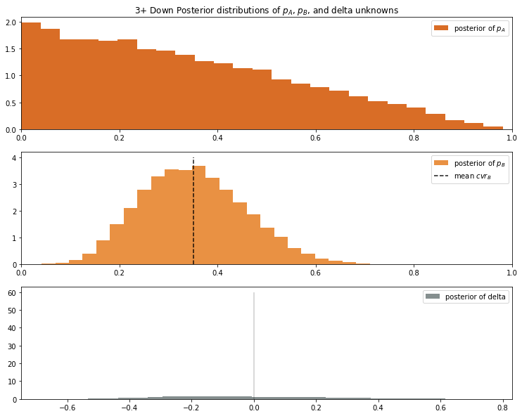
Accounting for the wider error margins, the probability of Collin Johson being the better receiver during a third down situation is 57%.
Appendix
Methodology
For this study, I started with Uniform distributions as my posteriors. I decided to go with NUTS as to produce the posterior sample. There wasn’t any major difference with Metropolis.
with pm.Model() as model:
    #prior
    p_A = pm.Uniform("p_A", 0, 1)
    p_B = pm.Uniform("p_B", 0, 1)

    # Deterministic delta function.
    delta = pm.Deterministic("delta", p_A - p_B)


    # Set of observations
    obs_A = pm.Bernoulli("obs_A", p_A, observed=observations_A)
    obs_B = pm.Bernoulli("obs_B", p_B, observed=observations_B)

    step = pm.NUTS()
    trace = pm.sample(20000, step=step)
    burned_trace=trace[1000:]
Validation
For those who need the converge tests…
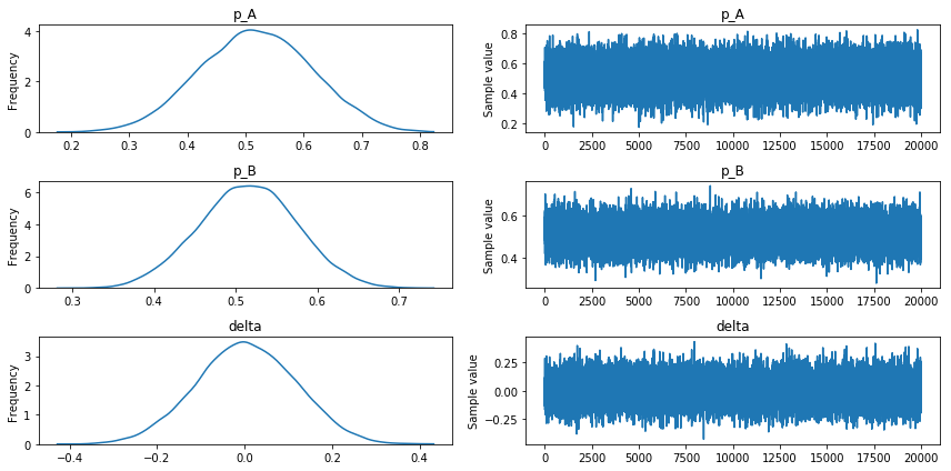
All Downs Convergence data
Third & 4th Down Convergence data
Our sample traces look to converge in a similar way as the ‘All Downs’ convergence data.
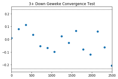
Since, we are dealing with reduced sample sizes and I’m dubious about the results. Let’s also run a Geweke convergences test.
Geweke convergence test checks differences means and variances at different parts of the same chain. PyMC3 allows you to pull the z-scores from the geweke function very easily. We will reject conversion if the majority of the points in the below plot, land 2 standard deviations from 0.
with model:
    start = pm.find_MAP()
    step = pm.Metropolis()
    trace_mp = pm.sample(5000, step, start=start)

z=pm.geweke(trace_mp, intervals=15)
plt.scatter(*z['delta'].T)
plt.hlines([-0.232,0.232],0,2500, linestyles='dotted')
plt.xlim(0,2500)
plt.title("3+ Down Geweke Convergence Test")