
Recruiting is the essence of College Football. It is one of the most important factors, if not the most important factor that determines how good a season will be. With this in mind, I dug up some data from 247Sports to see if we could use public recruiting event data to see if we could predict where a player was committing to, or at the very least see if a school of (my) interest was doing a good job at recruiting.
Summary of 2018 Recruiting
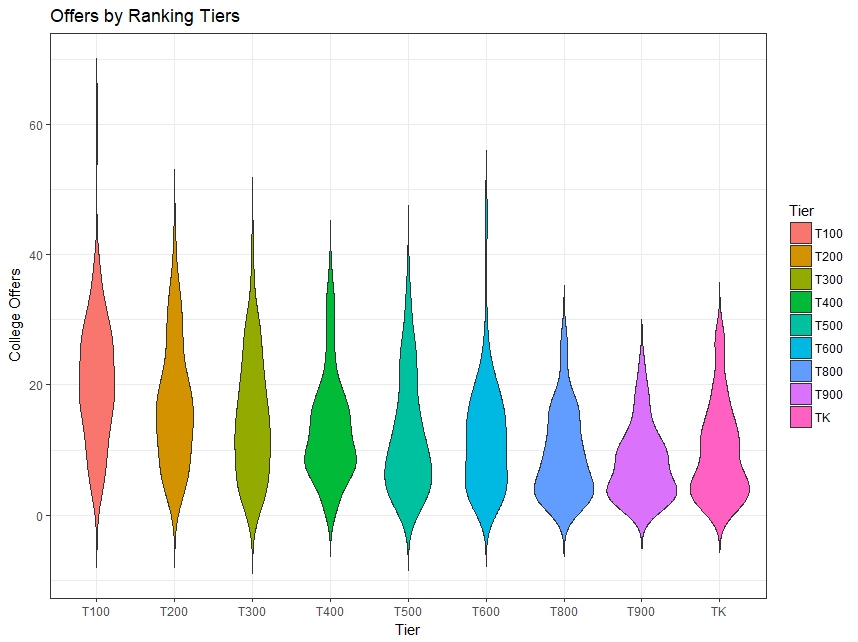
On average, recruits receive 13 offers. As we would expect, the higher the recruit is ranked, the more offers he might receive. In the chart below I grouped recruits by 100s according to their rank.
During the recruiting process, students get invited to schools (both officially and unofficialy), coaches visit students, and studentets attend summer camps. There are other events in the process but these 4 are the most consistent events documented in our source. So This analysis will be based on just those.
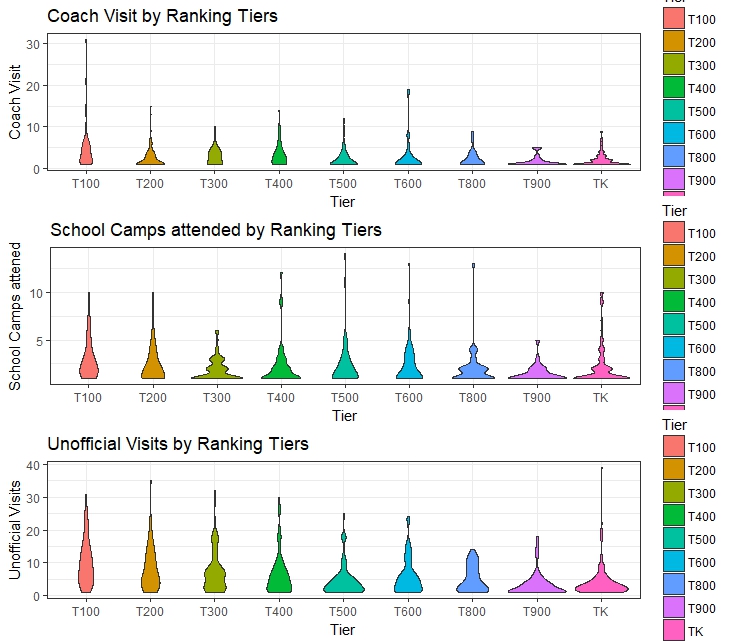
MEAN 2.32 School Visits, 6.19 Unoficial Visits, 1.97 Official Visits, 3.04 Coach Visits
As we can see, the top 100 tend to get the most love, but that doesn’t mean a ranked 999 recruit doesn’t get any attention.
Top FIVE Schools
Looking back at the 2018 class, Clemson, Georgia, Ohio State, Texas and USC finished in the top 5.
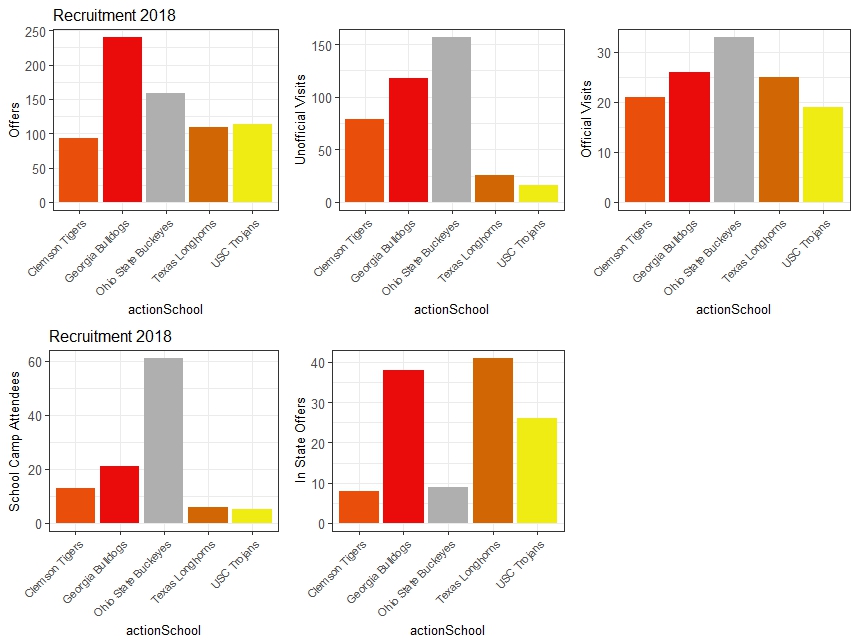
Georgia putting 200+ offers is the first thing that I noticed. UGA dropped over 200 offers when the average of the remianing Top 5 schools was 100. So much for OKG (Our Kind of Guy) for Coach Kirby huh. Second thing I noticed was Ohio State dominating in getting recruits to their campus on visits and School camps.
Modeling
Using the recruiting event data, let’s see if we can create a model to help us gauge where a recruit will end up playing.
Again, the recruiting events tracked are:
- Offer
- School Camp
- Unofficial Visit
- Official Visit
- Coach Visit
After extensive data manipulations, I create at table where each row represents a unique recruit and school that interacted with him. The metric columns (other than rank, in_state, and won) are the sum of events.
  name        actionSchool                 rank offer schoolCamp uvisit cvisit ovisit commits decommits in_state   won
  <chr>       <fct>                       <dbl> <int>      <int>  <int>  <int>  <int>   <int>     <int>    <dbl> <int>
1 Aaron Brule Cincinnati Bearcats           496     1          0      0      0      0       0         0        0     0
2 Aaron Brule Georgia Bulldogs              496     1          0      1      0      0       1         1        0     0
3 Aaron Brule Georgia Tech Yellow Jackets   496     1          0      0      0      0       0         0        0     0
4 Aaron Brule Mississippi State Bulldogs    496     1          1      0      0      1       1         0        0     1
5 Aaron Brule Oklahoma State Cowboys        496     1          0      0      0      1       0         0        0     0
6 Aaron Brule TCU Horned Frogs              496     1          0      0      0      1       0         0        0     0
The Method
I’m going to use a Logistic Regression Model, which would output the probability of a recruit commiting to a School.
\( P = h_{\theta(X)} = \sigma(\theta^{T}) X \)
Where the logit is:
\(logit[\pi(X)] = \beta{1}X_{SC} + \beta_{2}X_{oVisit}+ \beta_{3}X_{uVisit}+ \beta{4}X_{cVisit}+ \beta_{5}X_{inState} \)
The Prediction
model <-glm(won~schoolCamp+uvisit+cvisit+ovisit+in_state,
            family=binomial(link='logit'),data=training,
            control = list(maxit = 50))

summary(model)
Call:
glm(formula = won ~ schoolCamp + uvisit + cvisit + ovisit + in_state,
    family = binomial(link = "logit"), data = training, control = list(maxit = 50))

Deviance Residuals:
    Min       1Q   Median       3Q      Max
-2.8262  -0.1343  -0.1343  -0.1343   3.0703

Coefficients:
            Estimate Std. Error z value Pr(>|z|)
(Intercept) -4.70429    0.12495 -37.648  < 2e-16 ***
schoolCamp   0.52197    0.18353   2.844  0.00445 **
uvisit       0.23327    0.05058   4.612 3.99e-06 ***
cvisit      -0.13102    0.08994  -1.457  0.14518
ovisit       4.22311    0.14542  29.040  < 2e-16 ***
in_state     1.29659    0.17052   7.604 2.88e-14 ***
---
Signif. codes:  0 ‘***’ 0.001 ‘**’ 0.01 ‘*’ 0.05 ‘.’ 0.1 ‘ ’ 1

(Dispersion parameter for binomial family taken to be 1)

    Null deviance: 3143  on 7079  degrees of freedom
Residual deviance: 1620  on 7074  degrees of freedom
AIC: 1632

Number of Fisher Scoring iterations: 7
From the coefficients above, we can see why coaches (and fans mostly) get excited when recruits do official visits. This is not too surprising as the NCAA only allows 5 official visits per student. Unofficial visits are good indicators as well, althought they are not quite as strong. Summer Camps on the other hand seem to be very effective in the recruiting journey. Also interesting to me is the strength of the in_state coefficient. As a Texas fan I’ve heard much talk about keeping in state athletes home. The fact that this is the second strongest coefficient shows Texas isn’t the only school emphasizing on this point.
Now the question.. how good is this model? Overall, accuracy is at 95.56%, but I must admit this data is heavily skewed towards not winning a recruit.
predict<-predict(model,testing,type='response')
table(testing$won, predict > 0.5)
    FALSE TRUE
  0  5486   44
  1   218  152
As the last part of this analysis, I tried using the top 5 school (Texas, Georgia, USC, OSU, and Clemson) to see if they carried could help improve the regression analysis. Unfortunatley after several hours of feature engineering I couldn’t improve the model.
The simplest regression including schools as factors, shows Texas is the only school that can brag about being a significant factor.
> summary(model)

Call:
glm(formula = won ~ schoolCamp + uvisit + ovisit + in_state +
    TEX + USC + CLE + OSU + GA, family = binomial(link = "logit"),
    data = training, control = list(maxit = 50))

Deviance Residuals:
    Min       1Q   Median       3Q      Max
-3.3269  -0.1288  -0.1288  -0.1288   3.0969

Coefficients:
            Estimate Std. Error z value Pr(>|z|)
(Intercept) -4.78724    0.12926 -37.035  < 2e-16 ***
schoolCamp   0.36336    0.18779   1.935   0.0530 .
uvisit       0.27680    0.05157   5.368 7.98e-08 ***
ovisit       4.23948    0.14461  29.317  < 2e-16 ***
in_state     1.26161    0.17415   7.245 4.34e-13 ***
TEX          1.10482    0.45379   2.435   0.0149 *
USC         -0.11298    0.55735  -0.203   0.8394
CLE          0.62129    0.54551   1.139   0.2547
OSU          0.76816    0.46793   1.642   0.1007
GA           0.01940    0.41965   0.046   0.9631
---
Signif. codes:  0 ‘***’ 0.001 ‘**’ 0.01 ‘*’ 0.05 ‘.’ 0.1 ‘ ’ 1

(Dispersion parameter for binomial family taken to be 1)

    Null deviance: 3165.2  on 7079  degrees of freedom
Residual deviance: 1588.7  on 7070  degrees of freedom
AIC: 1608.7

Number of Fisher Scoring iterations: 7
Conclusion
Recruiting is tough for both recruits and schools (and fans!). Predicting where a player will commit and enroll is perhaps just as tough. I do think Texas is doing an outstanding job at recruiting, and unlike Georgia, Texas is being selective in who gets an offer. The idea of getting the best players from within the state worked well for the Texas 2018 recruiting class. However, not all states are as big as Texas, and not all states have the same football talent as Texas so it might be hard for other schools copy this model and be succesful.