
In this post, I’m testing a popular soccer metric, Pass Ratio (PR), with NFL passer/receiver data and I’ll try to determine if this metric can help predict total air yards produced by an offense.
Pass Ratio was first developed by the mathematicion Thomas Grund. He used it to evaluate soccer matches and discovered that teams that focused their passing on a select few players usually scored less goals than teams who distributed their passes evenly. It is important to note that soccer has a more complex pass network as all players receive and pass the ball. There are some players analogous to football’s QB, who tend to distribute the ball the most (center midfield), but the rest of the team does their fair share of passing. Football, as we know, only the QB passes the ball. Ocassionaly, a RB or a kicker may throw the ball on a trick play, but let’s ingore those cases as they are not frequent.
The motivation to test this metric, is that if a QB does his receiver progressions well, and has multiple players able to separate from their coverage, then that QB would be passing to multiple targets and possibly having a better offense. If a QB only trusts a select group of receivers , then the opposing defense should be able to double cover those safety targets and reduce the effectiveness of the offense.
Calculating Pass ratio for NFL :
As mentioned before, the Pass Ratio is a way to measure network centrality at a game level. This metric is calculated by counting the number of times of a player received the ball. We find who received the ball the most, and use his reception number as the game max. We then calculate the difference in passes by subtractig each players passing count from the game max. We average the differences of all players, and finally divide them by the total number of passes completed in the day. This will result in a number ranging between 0 and 1.
\(MPD = \frac{\sum_{i=1}^{TP} maxPasses - passes_i}{TP} \)
\(PR = \frac{MPD}{TotalPasses} \)
Where:
- TP: total number of receivers who caught a pass during the game
- maxPases: the highest number of passes thrown at one person during the game
- TotalPasses: Total passes thrown by the QB
For eaxmple: Dak throws to Dez 15 times, 10 times to Witten and 5 times to Beasley. Our calculations will go as this.
\( Mean Pass Diff = \frac{(15-15)+(15-10)+(15-5)}{3} = \frac{0+5+10}{3} = \frac{15}{3}=5 \)
\( \frac{5}{15+10+5} = \frac{5}{30} = 0.1666667 \)
\(PR = 0.17 \)
If a QB throws at multiple targets in an even distribution, then his team’s pass ratio will be rather low. Alternatevely, if a QB, caves in to his diva WR and makes every pass to him, then his team will have a high PR.
Analysis
Analysis is rather simple, just a linear regression with PR as the independent variable, and Pass Yards as the dependent variable. I decided to compare PR to total pass yards, meaning air yards AND yards after completion. My argument, is that if a team distributes it’s passes evenly throught receivers, then eventually a receiver will catch a pass and have plenty of room to run after the catch as the defense would be spread out accross the field.
Game by Game
By simply plotting the data, it is difficult to say there is a linear relation.
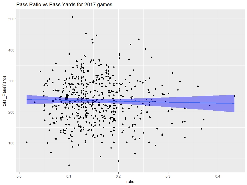
R squared is essentailly 0.
>lr_model<-lm(formula=total_PassYards~ratio,data=game_pr
>summary(lr_model)
Call:
lm(formula = total_PassYards ~ ratio, data = game_pr)

Residuals:
     Min       1Q   Median       3Q      Max
-208.684  -52.124   -2.148   51.195  269.528

Coefficients:
            Estimate Std. Error t value Pr(>|t|)
(Intercept)  239.659      8.462  28.322   <2e-16 ***
ratio        -29.750     50.094  -0.594    0.553
Test at Season Level
PR at a game level is a horrible predictor. I still have hope though. Maybe game-by-game is too granular and PR should considered as an average metric. Maybe QBs/Receivers have bad days and catch the ball but cant transform them into yards.
I grouped the data to represent mean(PR) and mean(Total Pass Yards).
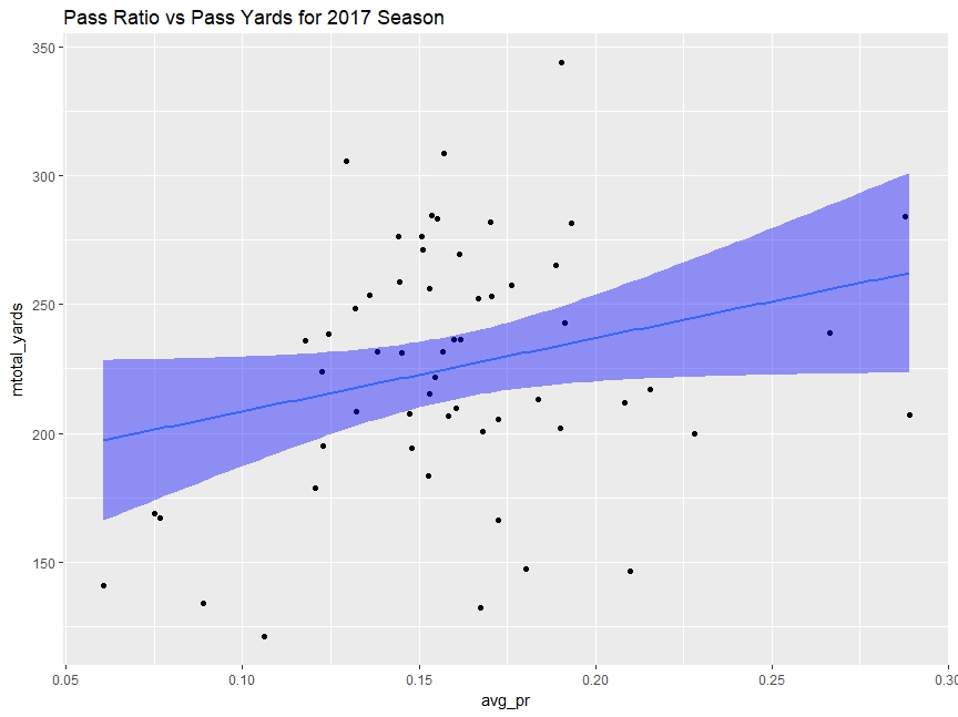
The trendline shows a positive relation, but we can easily tell it is a horrible fit. Again, R squared is close to 0.
> lr_model<-lm(formula=mtotal_yards~avg_pr,data=season_pr)
> summary(lr_model)

Call:
lm(formula = mtotal_yards ~ avg_pr, data = season_pr)

Residuals:
    Min      1Q  Median      3Q     Max
-95.111 -28.045   7.228  31.253 109.802

Coefficients:
            Estimate Std. Error t value Pr(>|t|)
(Intercept)   180.02      23.67   7.605 3.85e-10 ***
avg_pr        284.41     142.48   1.996   0.0509 .
---
Signif. codes:  0 ‘***’ 0.001 ‘**’ 0.01 ‘*’ 0.05 ‘.’ 0.1 ‘ ’ 1

Residual standard error: 46.81 on 55 degrees of freedom
Multiple R-squared:  0.06755,	Adjusted R-squared:  0.0506
F-statistic: 3.985 on 1 and 55 DF,  p-value: 0.05088
Just for fun
Now, just for fun, I’ll look at the residual fits.
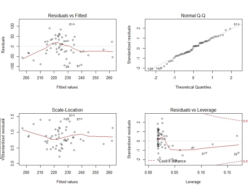
- Residuals vs Fitted: there is no distinctive pattern, so I’ll it’s safe to call this a linear relationship.
- Normal Q-Q plot: looks like a stright line, I can validate the errors follow a normal distribution.
- Scale-Location: In this graph we test our assumption of equal variance (homoscedasticity). At simple glance, points look equaly spread out, so nothing werid here
- Residual vs Leverage: Nothing really outside Cook’s distance, thus there’s no single point hurting my regression
Conclusion
At this point, I think continuing with this excersie is moot. While PR is a good predictor in soccer, it just doesn’t transfer well to football. Perhaps, the ability of some WRs compensate and justify them getting more passes. Also, it might be the case that when you target different players evenly, you just don’t have the super star WR. Either way, I’ll remove PR form my key metrics.